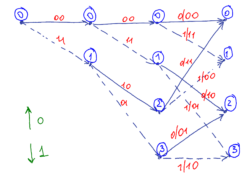
Introduction

The Forward-Backward algorithm with some modifications can be used for decoding on a trellis. This algorithm is known as BCJR and was introduced in [1]

Our Model

Let’s take a look again to a trellis

An encoder uses an input symbol(green) to generate a codeword symbol (red) based on current state. Then the Encoder updates its state and pushes the codeword symbol into a channel or, in terms of HMM world, encoder emits.

The channel corrupts the symbols during transmission. Receiver observes noisy codewords or, it terms of HMM worlds, decoder observes.

Now the decoding task can be expressed in terms of HMM as follows: What is a codeword at sender, that could “most likely” produce the received sequence given known channel conditions?

The main difference between BCJR and Fast-Forward algorithm is that emissions in HMMs appear only in states. But in a trellis, emissions appear during the transitions(!) between states.

Emission probability matrix

In case of hard-decoding, emissions are discrete and an emission probability matrix has a finite number of elements. \(O_t\) is a number of all possible received symbols.

In case of soft-decoding, emissions and corresponding \(B\) matrix are continuous variables. We may still notice, that the computation model remains the same: taking into an account, that trellis produces only on possible emission during state transition, we may write: \(\begin{aligned}P(O^t \mid S^t, S^{t+1}) & = \sum_{E^{l}} P(O^t, E^l \mid S^t, S^{t+1}) = \\ & = \sum_{E^{l}} (P(O^t \mid E^l, S^t, S^{t+1}) * P(E^l \mid S^t, S^{t+1})) = P(O^t \mid E^t) = \\ & = \prod\limits_{i} P(O^t(i) \mid E^t(i)))\end{aligned}\)

, where: \(\begin{aligned}P(O_t(i) \mid E_t(i)) = \begin{cases} {\displaystyle {\frac {1}{\sigma {\sqrt {2\pi }}}}e^{-{\frac {1}{2}}\left({\frac {r(i)-\mu }{\sigma }}\right)^{2}}}, & \text{if } S^t(i)=0.\\ {\displaystyle {\frac {1}{\sigma {\sqrt {2\pi }}}}e^{-{\frac {1}{2}}\left({\frac {r(i)+\mu }{\sigma }}\right)^{2}}}, & \text{otherwise}. \end{cases}\end{aligned}\)

• \(E^t(i)\) - i-th bit of codeword, produced by state transition from \(S^t\) to \(S^{t+1}\)
• \(O^t(i)=r(i)\) - received value

Algorithm description

Now, \(\alpha\)’s are computed using following steps:

1. Step 1: \(\alpha_{0}(i)= \pi(S_{i})\)
2. Step \(t+1\): \(\alpha_{t+1}(i)= \sum\limits_{j =1} \alpha_{t}(j) \cdot P(S^{t+1}_{i} \mid S^{t}_{j}) \cdot P(O^{t} \mid S^{t}_{j}S^{t+1}_{i})=\\= \sum\limits_{j =1} \alpha_{t}(j) \cdot P(S_{i} \mid S_{j}) \cdot P(O^{t} \mid S_{j}S_{i}) = \\=\sum\limits_{j =1} \alpha_{t}(j) \cdot \gamma_{t}(ij)\)

We would note here:\(\alpha_{t}(i) = P(O^{1} \dots O^{t}, S^{t+1} = i)\)

Now, \(\beta\) are computed using following steps:

1. Step 1: \(\beta_{L+1}(i)=1\)
2. Step 2: \(\beta_{t}(i) = \sum\limits_{j =1}^{N} P(S^{t+1}_{j} \mid S^{t}_{i}) \cdot P({O^{t}} \mid S^{t}_{i}S^{t+1}_{j}) \cdot \beta_{t+1}(j)=\\=\sum\limits_{j =1}^{N} P(S_{j} \mid S_{i}) \cdot P({O^{t}} \mid S_{i}S_{j}) \cdot \beta_{t+1}(j)\)

We may also note: \(\beta_{t}(i) = P(O_{t} \dots O_{L} \mid S^{t} = S_{i})\)

Similary to what we’ve done in Forward-Backward algorithm , we may write: \(\begin{aligned}&P(S^t = i, S^{t+1} = j \mid O^1 \dots O^L) = \\ &= \frac{P(O^1 \dots O^{L} \mid S^t = i, S^{t+1} = j) \cdot P(S^t = i, S^{t+1} = j)}{P(O^1 \dots O^{L})} = \\ & = \frac{P(O^1 \dots O^{t-1} \mid S^t = i) \cdot P(O^{t} \mid S^t = i, S^{t+1} = j) \cdot P(O^{t+1} \dots O^{L} \mid S^{t+1} = j) P(S^t = i, S^{t+1} = j)}{P(O^1 \dots O^L)} = \\ &= \frac{\frac{P(O^1 \dots O^{t-1}, S^t = i)}{S^t = i} \cdot P(O^{t} \mid S^t = i, S^{t+1} = j) \cdot P(S^t = i, S^{t+1} = j) \cdot \beta_{t+1}(j)}{P(O^1 \dots O^L)} = \\ &= \frac{P(O^1 \dots O^{t-1}, S^t = i) \cdot \frac{P(O^{t}, S^t = i, S^{t+1} = j)}{S^t = i} \cdot \beta_{t+1}(j)}{P(O^1 \dots O^L)} = \\ &= \frac{\alpha_{t-1}(i) \cdot P(O^{t}, S^{t+1} = j \mid S^t = i) \cdot \beta_{t+1}(j)}{\sum\limits_{i} \alpha_{t}(i) \beta_{t}(j))} = \\ & =\frac{\alpha_{t-1}(i) \cdot P(O^{t}\mid S^t = i, S^{t+1} = j) P(S^{t+1} = j \mid S^t = i ) \cdot \beta_{t+1}(i)}{\sum\limits_{i} \alpha_{t}(i) \beta_{t}(j))}= \\ &= \frac{\alpha_{t-1}(i) \cdot \gamma_{t}(ij) \cdot \beta_{t+1}(j)}{\sum\limits_{i} \alpha_{t}(i) \beta_{t}(j))}\end{aligned}\)

Note: in literature \(\alpha\) can start with different index

And few remarks…

We can raise the following questions:

Q: Emission matrix \(B\) now depends on time. Will it affect the computations using Forward-Backward Algorithm? A: No :-)

References

1. L. Bahl, J. Cocke, F. Jelinek, and J. Raviv, “Optimal decoding of linear codes for minimizing symbol error rate (Corresp.),” IEEE Trans. Inform. Theory, vol. 20, no. 2, pp. 284–287, Mar. 1974, doi: 10.1109/TIT.1974.1055186.

Last update:14 November 2021